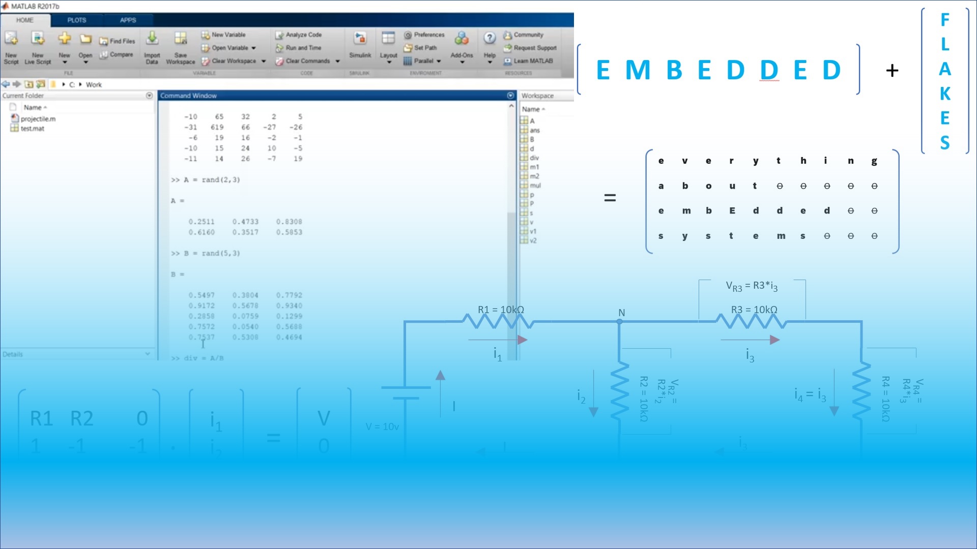
Matrix is very versatile mathematical tool used in diverse fields like robotics, machine learning, mechanics, electronics and so on. In this article, we are going to see different operations we can do with vectors and matrices in MATLAB.
MATLAB itself stands for MATrix LABoratory. All MATLAB variables are arrays. Each variable can contain multiple numbers. Most MATLAB functions work on multiple values at once.
Type of Vectors and Matrices
Let’s look at the different type of arrays are used in MATLAB
A matrix is an array with multiple rows and multiple columns.
A scalar means a matrix with a single element. A scalar is a single number that is essentially a one-by-one array.
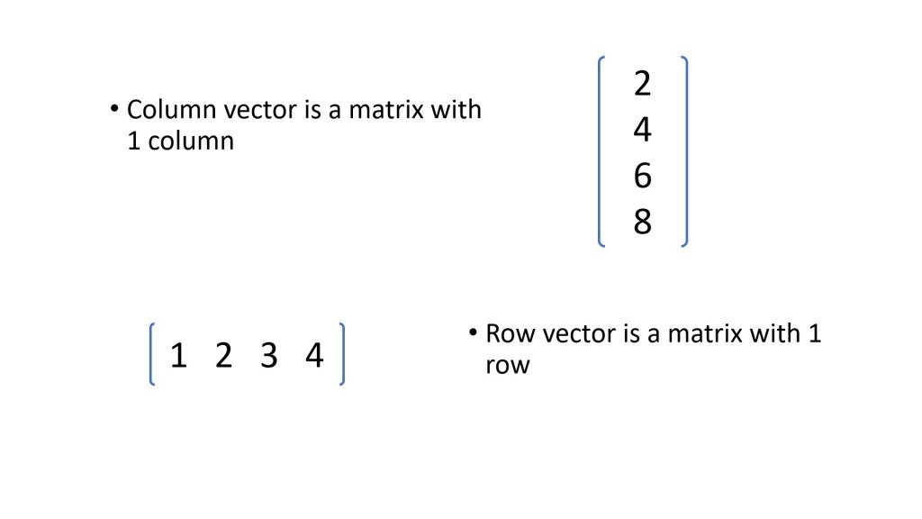
A column vector is a matrix of single columns and multiple rows.
A row vector is a matrix with a single row and multiple columns.

Creating Vectors Manually
We can create a matrix or array using square brackets. If numbers within the square brackets are separated by space or comma, then MATLAB creates a row vector. If numbers are separated by semicolons then MATLAB creates a column vector.
>> Row1 = [1 2 3 4 5]
>> Row2 = [10,20,30,40,50]
>> Col1 = [1;2;3;4;5]
Spaces and semicolons combined to create a matrix. A matrix is entered row by row where each row is separated by a semicolon.
>> m = [1 2 3; 4 5 6; 7 8 9]
Evenly spaced vectors are very common. It is not practical to enter long vectors manually. MATLAB gives a shorthand method to create evenly spaced vectors. Use colon operator and specify starting and ending points.
>> even_row = 5 : 8 create a row vector with elements 5, 6, 7, 8.
The colon operator uses a default spacing of 1. We can specify different spacing using the colon operator.
>> even_row = 20 : 2 : 30 creates a row vector with elements 20, 22, 24, 26, 28, 30.
>> even_row = 1 : 0.5 : 5 creates a row vector with elements 1.0, 1.5, 2.0, 2.5, 3.0, 3.5, 4.0, 4.5, 5.0.
Another method to create evenly spaced vectors is the linspace() function. We must specify the number of elements we want in a vector.
>> even_row = linspace(0, 1, 5) creates a row vector with 5 elements evenly spaces from 0 to 1.
So far we created row vectors. How can we create column vectors? We can create column vectors manually, by entering the elements and separating them by a semicolon.
>> col1 = [2; 4; 6; 8; 10]
Another method is to create a row vector using one of the shorthand methods discussed before and then use the transpose operator to create a column vector.
>> even_col = even_row'
Vector and Matrix Creation Functions
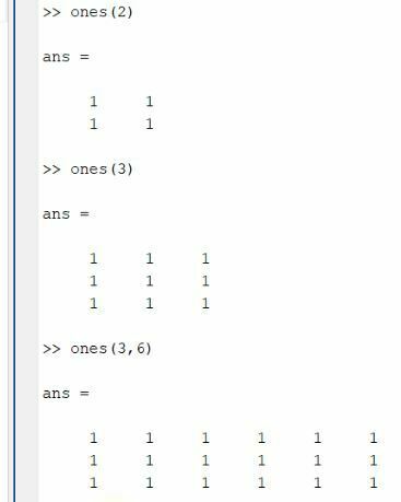
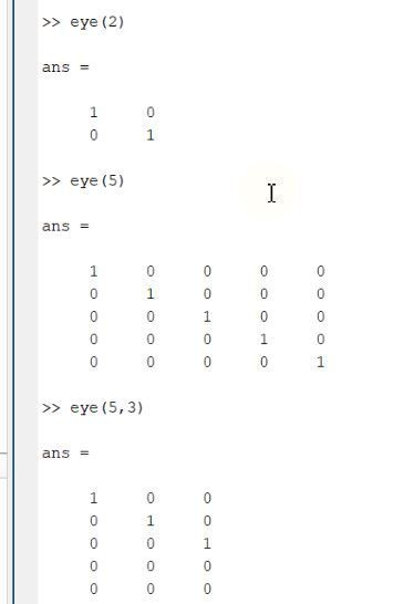
We can quickly create a square or non-square matrix using random numbers. Ones() and zeros() can be used to create an array of all ones and an array of all zeros. eye() function is used to create identity matrix. diag() function can be used to create a diagonal matrix or to get diagonal elements of a matrix.



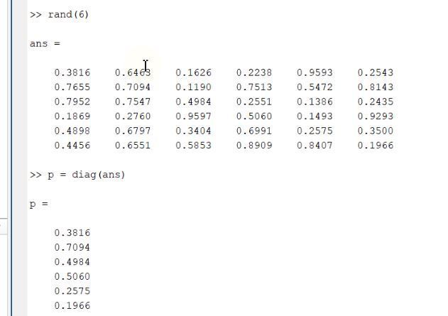
Size() function gives the size of a vector or a matrix.

Indexing
The position of an element in a matrix or array is called its index. We can use an index to extract or modify a particular element.
For Matrix, an element belongs to row r and column c then (r,c) becomes its index.
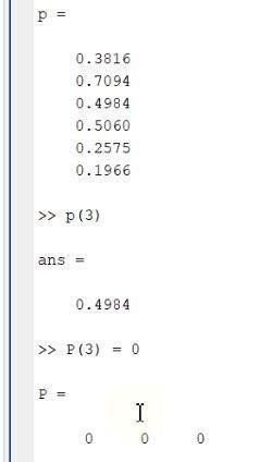

We can read or modify a whole row or a whole column using colon operator. Use the end keyword to refer to the last element.
>> x = v(1, : ) reads entire 1st row.
>> x = v(: , end) reads entire last column.
The range of values in an array or a matrix can be accessed using a colon operator.
>> x = v(2:4, 3) reads elements 2 to 4 in 3rd column.
Array Arithmetics
Array operations are executed element by element. We can add or subtract a scalar value to each element of a matrix. Multiply or divide an array with a scalar value. Element by element product of matrix A and matrix B is done by element-wise multiplication operator “.*”.
if two arrays/ matrix are of the same size then each element in the first operand is matched with the corresponding element in the second operand to perform arithmetic. for example, we can add two vectors of the same size.
>> A = [1 2 3];
>> B = [2 2 2];
>> A+B
>> ans =
3 4 5
If we want to perform arithmetic operation of a scalar to a matrix, MATLAB implicitly converts scalar to the same size as the matrix. for example,
>> A = [1 2 3; 4 5 6];
>> 4 .* A
>> ans =
4 8 12
16 20 24
If size of two matrix is incompatible the MATLAB throws an error.
Below table gives summary of array arithmetic operators available in MATLAB.
| Operator | Function | Description |
| + | Addition | Adds two matrices of the same size. for example, A+B adds A and B. |
| + | Unary plus | Returns the same matrix. for example, +A returns A. |
| - | Substraction | Substracts the second matrix from the first. for example, A-B subtracts B from A. |
| - | Unary minus | Returns negative matrix. for example -A negates the elements of A. |
| .* | Element wise multiplication | A .* B returns the element-wise product of A and B. |
| .^ | Element wise power | A .^ B raises each element of A to the corresponding power in B. |
| ./ | Right array division | A ./ B divides each element of A by the corresponding element of B. |
| .\ | Left array division | B .\ A divides each element of A by the corresponding element of B. |
| .’ | Array transpose | A .’ returns the non-conjugate transpose of A, that is, interchanges the row and column index for each element. |
Matrix Arithmetics
Matrix operations are done as per linear algebra rules. The required size of the input matrix depends on the operation. To do matrix multiplication with matrix multiplication “*” operator the matrices must have a common inner dimensions. This means the number of columns in the first matrix must be equal to the number of rows in second matrix. In order to divide matrix, A divide by matrix B using right division operator “/”, the matrices A and B must have the same number of columns.
Below table provides summary of matrix operators available in MATLAB.
| Operator | Function | Description |
| * | Matrix multiplication | A * B is the matrix product of A and B. If A is an m-by-p and B is a p-by-n matrix, then C is an m-by-n matrix defined by. For nonscalar A and B, the number of columns of A must equal the number of rows of B. Matrix multiplication is not universally commutative for nonscalar inputs. That is, A*B is typically not equal to B*A. |
| \ | Matrix left division | A \ B solves the system of linear equations A*x = B. The matrices A and B must have the same number of rows. |
| / | Matrix right division | B / A solves the system of linear equations x*A = B for x. The matrices A and B must contain the same number of columns. |
| ^ | Matrix power | A ^ B computes A to the B power. |
| ‘ | complex conjugate transpose | The complex conjugate transpose of a matrix interchanges the row and column index for each element, reflecting the elements across the main diagonal. The operation also negates the imaginary part of any complex numbers. |
Application of Matrix in Circuit Analysis
Now, let’s see one application of the matrix.
Analyze the circuit and find currents flowing through the different resisters.

Here we will use Kirchoff’s laws, which states that
- the total change in electrical potential around a closed loop is zero.
- The sum of all currents at any node in teh circuit is zero.
The potential difference across resistor R1 is i1R1 and the Potential difference across register R2 is i2R2.
Then according to the 1st law, we get
i1R1 + i2R2 = V
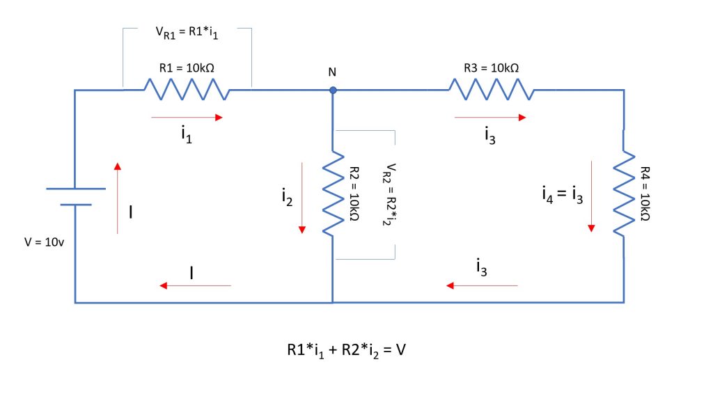
At node N, the current flowing in is i1 and currents flowing out are i2 and i3.
Then as per 2nd law, we get
i1 - i2 - i3 = 0

Potential difference accross resister R2 is same as sum of potential difference across R3 and R4.
i2R2 = i3R3 + i3R4
therefore
-i2R2 + i3R3 + i3R4 = 0

these linear equations can be arranged in matrix format Z.i = v
therefore i = Z-1 .v
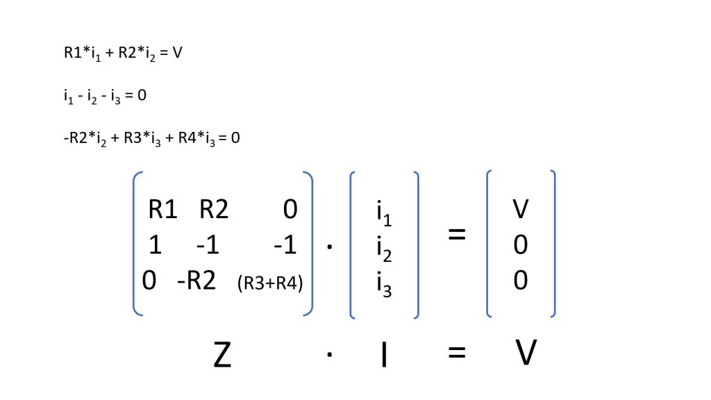
To solve linear equations in matrix format, use linspace() function.


